
How to Use LOOKUP in Google Sheets: Google Sheets works best as a database holding vast amounts of information in the form of spreadsheets and workbooks. It can be used to deal with basic functionalities to store data and manipulate and retrieve it as and when required. If you know about Advanced Excel, you must have come across the word LOOKUP.
The LOOKUP function basically helps us find specific information from a set of data. Let’s dive quickly into the topic to learn more about the LOOKUP using Google Sheet tips and its functionalities. Scroll down to find out more.
- How To Use Lookup Function in Google Sheets?
- Google Sheets Lookup Multiple Criteria
- How To Use Vlookup in Google Sheets?
- How To Use Vlookup in Google Sheets From a Different Sheet?
- Using Hlookup in Google Sheets
- How To Put Search Box In Google Sheets?
- How To Use the Find Function in Google Sheets?
- How To Use Match Function in Google Sheets?
- How To Hide Google Sheets Formula?
- Limitations of Lookup Google Sheets
- FAQs LOOKUP in Google Sheets
How To Use Lookup Function in Google Sheets?
LOOKUP is a complicated function. This basically helps in fetching a piece of particular information from a set of considerably large amounts of data. Implementing this function for numbers is easy, but it can work very trickily with text. The basic syntax is: =LOOKUP( search_key, search_column, return_column), where:-
- Search_key represents the entity you are searching for
- Search_column refers to the location where you are searching
- Return_column represents the data you need.
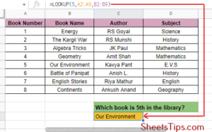
Let’s understand this better with an example. For example, we have a spreadsheet that represents the data of a list of textbooks in the school library. The information we are provided with is ID, name of the book, author, and subject.
Now, suppose we wish to find out which book has id number 5. So, the formula we need to put here is =LOOKUP( 5, A2: A9, B2: B9). This will return the value that is our environment in our case.
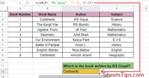
But, what if we want to search for a book by its author or subject’s name? This gets a little complicated here because we need to work with a text string and not a number. So, for example, we wish to search for a book that was written by RS Goyal.
For this, simply use the formula =LOOKUP( “RS Goyal”, C2: C9, B2: B9). Remember, a string always needs to be encompassed within double quotes.
Now, what if you don’t remember the surname of the author, Goyal, and you only know his first name, which is RS? But, searching with only RS won’t work here because you have multiple options with that command, so Google Sheets will end up giving you the wrong answer.
The symbol you need to use here is wildcard percent (%). Write RS%, which means that there is more text after that RS that is unknown to you.
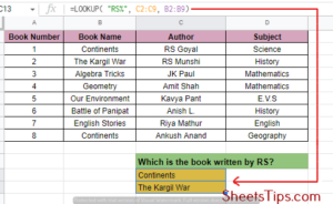
Thus, you use the formula =LOOKUP( “RS%”, C2: C9, B2: B9). Google Sheets shows the output for all the books written by authors having the first name as RS, and provides n/a as an output if there are none.
Google Sheets LOOKUP Multiple Criteria
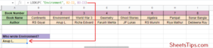
Previously, we learned how to use LOOKUP for columns in Google Sheets. But, are you wondering how to use LOOKUP for rows in Google Sheets with multiple criteria? Well, here it is.
The only change in the formula would be row cell ranges instead of column cell ranges. So, the final formula would be = LOOKUP( “RS Goyal”, B1: I1, B2: I2).
How To Use VLOOKUP in Google Sheets?
Lookup extends its functionalities by using VLOOKUP and HLOOKUP, which are basically twin daughter functions for LOOKUP. They are more convenient and problem-solving as compared to LOOKUP. Let’s learn about VLOOKUP first in this section.
VLOOKUP basically works for vertical compartments of data where it searches the first column of a range for an entity and returns it in the row it found. The syntax we use here is =VLOOKUP( lookup_value, range_array, column_index, is_sorted ), where:-
- lookup_value is the entity on which you want to perform the search.
- range_array is the total range of the table you are searching in.
- column_index is the column the value of which you want to fetch.
- is_sorted tells whether you want a true match that returns 0 or an approximate match that returns 1. If the range is sorted in ascending manner it returns 1, and if in descending it returns -1
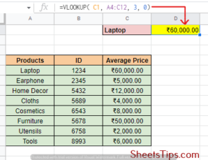
In this example, we are using a table that has products along with their ID and average price. Suppose we want to search for the average price of a product: laptops. Select a particular cell to write your lookup value. Here we have taken and on the cell you want to display the result, apply the formula =VLOOKUP( C1, A4:C12, 3, 0).
How To Use Vlookup in Google Sheets From a Different Sheet?
If we wish to use VLOOKUP to fetch certain data in a sheet from another workbook, then we can use the same old formula with just a little bit of change in the parameter combination.
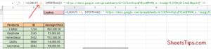
This is where the IMPORTRANGE function comes in. The syntax we use is =IMPORTRANGE( spreadsheet_key, range_string), where spreadsheet_key is the URL of the spreadsheet you want to import from and range_string is the cell range reference that we want to import.
- Step 1: Go to the cell of your current spreadsheet and click on the cell range where you want the LOOKUP value to display.
- Step 2: Next, type =VLOOKUP ( followed by the cell reference of the value you want to look up and a comma (,).
- Step 3: Now, navigate to the spreadsheet where you want to import the cell range and copy the URL to your clipboard.
- Step 4: Finally, add the formula =VLOOKUP( A3, IMPORTRANGE( ” range_URL” )) and hit Enter.
Using HLOOKUP in Google Sheets
HLOOKUP, or Horizontal LOOKUP, basically searches horizontal parts of data where it searches across the first row of a range for an entity and returns the value in the column it finds. The syntax we use here is similar to the VLOOKUP one that is =HLOOKUP( search_key, range_array, row_index, is_sorted ), where:-
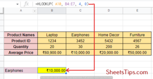
In this example, we are performing a search on a table that shows salon services along with the discounts going on them. If we want to find out what the current nail art discount offer is, we can select the search_key value cell and then apply the formula =HLOOKUP (A10, B4: E7, 4, 0) to the result cell.
How To Put Search Box In Google Sheets?
In this section, we will teach you how to insert a search box with a drop-down list in Google Sheets. Let’s see an example and see the steps to understand better.
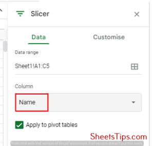
- Step 1: Select the entire table and click on Add a slicer from the data menu.
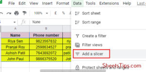
- Step 2: Go to the slider sidebar and select the value from the column where you need to search, Name here.
- Step 3: Select Filter by condition and choose Text contains from the drop-down list. Type 1 and click on OK.
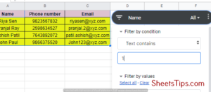
Now, you will only be shown the details of the entity you type on this search bar.
How to use the Find function in Google Sheets?
The FIND function in Google Sheets helps in fetching and returning the position where a string is first found. FIND is case-sensitive and works best for those cases where the return values are not matched. The syntax to be used is =FIND( search_for, text_to_search, starting_at), where search_for refers to the string we are looking for, text_to_search refers to the first occurrence of search_for, and starting_at is optional and refers to the character to search at and is set to 1 by default.
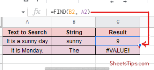
For example, we want to search if sunny is present in the sentence, It is a sunny day. The formula you should use here is =FIND(B2, A2). The result you get is 9 which is the index where the word starts. It will return #VALUE! if the searched word is not present in the given string.
How to use the MATCH function in Google Sheets?
The Match value in Google Sheets basically returns the relative position of an entity in a range that matches a particular value. MATCH returns the output in the form of an array or a range of matched values rather than a single value itself. The syntax used is =MATCH( search_key, range, search_type), where search_key is the value to search for, the range is the 1D array to be searched in, and the search type is 1, 0, or -1 accordingly.
If the search_type is 1, it indicates to the MATCH function that the array is sorted in ascending order and will return the largest value less than or equal to the search_key. If the search_type is 0, it represents an exact match for an unsorted array. And if the search_key is -1, it tells the MATCH function that the array is sorted in descending order and will return the smallest value greater than or equal to the search_key.
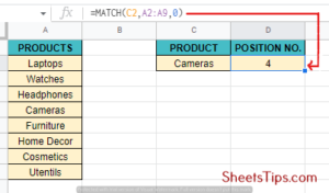
In this example, let’s consider a table having a student’s name, roll number, and their position in academics. Let’s say we want to find the class position of roll number 40. Select a cell to enter the search key, and then on the result cell, apply the formula =MATCH( A9, A2: A5, 0).
How To Hide Google Sheets Formula?
You can easily hide certain formulas after adding them to your spreadsheet. Not all, but in certain standard keyboard sets, there is a grave accent key present on the top left corner of the first key that looks like an inverted apostrophe. Use the key combination Ctrl+` as a toggle button that allows you to both show and hide the formulas on your spreadsheet.
Limitations of LOOKUP Google Sheets
Many users have reported their LOOKUP Google Sheets not working. LOOKUP is a very efficient function, but it might fail silently sometimes. To avoid this, you must incorporate small setups.
Your table must be sorted and free of man-made errors to allow LOOKUP to work smoothly. Also, try using Vlookup and Hlookup more because that gives you better control over your data.