Handling subjective data in Google Sheets necessitates the use of dates and times. We have already dedicated an article to you previously that talks about how to calculate days between two dates in Google Sheets. Now, you must be wondering how to add and subtract time in Google Sheets. Well, this is also very simple, and in this article we are going to discuss how to add time intervals in Google Sheets, timesheets, time tracking, adding time, setting time to 24-hour format, and other important Google Sheet tips, so make sure you read till the end to find out.
- How To Insert Time Stamp in Google Sheets Cell?
- How To Add Hours on Google Sheets?
- Add Minutes to Time in Google Sheets
- How To Add Seconds in Google Sheets?
- Set Google Sheets 24-Hour Time Format
- Convert Time to Number in Google Sheets
- Adding Time Tracker in Google Sheets
- FAQs
How To Insert Time Stamp in Google Sheets Cell?
Google Sheets provides us with a couple of formulas to achieve quick time and date retrieval. If you are wondering how to insert the current time in Google Sheets, then use the formula =NOW( ). To insert the current date, use the formula =TODAY( ). So, if you are wondering how to add a date and time in Google Sheets, use these formulas.
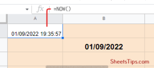
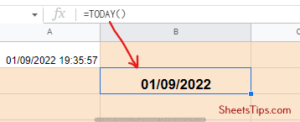
As we know, these formulas are volatile; they will change as you change the cell address. If you set the formula for current and come check it the next day, then you will get an updated result. So, to get proper timestamps on your Google Sheets page, you will have to make these formulas static. The formula that is going to automatically insert time stamps for you in Google Sheets is Apps Script. Let’s see the steps:
- Step 1: Go to your Google Sheets document and click on the Extensions option from the menu. Click on the drop-down menu that appears, and click on the “Apps Script” option.
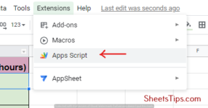
- Step 2: When the Apps Script code window opens, copy-paste the following code that we have taken from Stackoverflow:
- Step 3: Next, click on the Save icon to save this code. Once that’s done, whenever you enter some data in a particular column, you will see its timestamp in the adjacent column.
If you don’t want to go through so many steps, you can also opt for a keyboard shortcut for the same. To insert the current date, press the key combination Ctrl+Colon (or 🙂. To insert the current time, press the keys Ctrl+Shift+Colon (or 🙂 together.
To display the date and time together, first, use the keyboard shortcuts mentioned above and then add them. You can also achieve this by using the keyboard shortcut Ctrl+Shift+Alt+;, as shown below.
Apart from this, you can also use the SPLIT function to extract the date in one cell and the time in another one because the timestamp is composed of both the date and the time. In the result cell B2, type the formula =SPLIT(A2, “”) and hit Enter.
This will automatically enter the date separately in cell B2 and the time in cell C2. Next, click on the fill handle plus icon to fill this formula across the entire column of B.
How To Add Hours on Google Sheets?
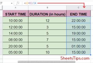
Consider that you are working with a data set that looks something like what we have mentioned below and has a date and time to work with. So, if you want to add hours to the time, you can’t just do it like you’re adding dates.You will first need to make sure that the units of the columns are similar and in the 24-hour format. So, if your time is in the 24-hour format, then you can achieve the correct result just by adding the hours and dividing them by 24.
For better understanding, look at the screenshot shared above where we have used the formula =A2+B2/24. One thing you need to note here is that if you add long hours, like above 20 or more, then it will shift to the next day and you will be shown the time of the next day.
How To Add Minutes to Time in Google Sheets?
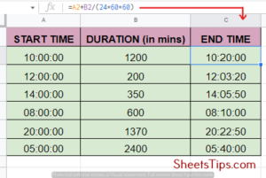
Before adding minutes to the time mentioned, you must ensure that the unit of the time mentioned in the values you want to add is the same as the time entered—that is, minutes.
Take the following dataset as shown below, for example, where you want to add time in minutes given in column B to the values previously entered in column A. To enter the result, create a new column, say C, and use the formula =A2+B2/(24*60). Finally, to convert this value from column B to minutes, divide it by (24*60).
How To Add Seconds in Google Sheets?
Just like adding hours and minutes, adding seconds is also very simple here. Firstly, make sure that the unit of the time in your time column header needs to be the same as the unit of the values being added, that is seconds.
From the following example, consider you are working with a time dataset as shown below and want to add the second value in column B to the time entered in column A.
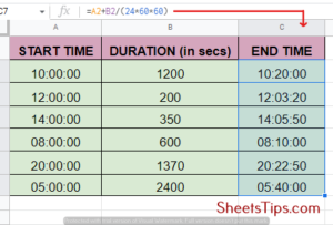
Simply create a new end time column in C2 and enter the formula =A2+B2/(24*60*60). Drag it till the end with the help of the fill handler to apply the formula to the entire column. Finally, make sure you don’t forget to convert the value in Column B into seconds by simply dividing it by (24*60*60) and you are ready with your new end time data.
How To Set Google Sheets 24-Hour Time Format?
Every human being has their own preferences when it comes to daily necessities, one of which is time. If you want to custom format the time cells according to your choice, which can be 24 hours or more, follow the steps shown below:
- Step 1: Select all the cells for which you wish to customize and change the cell format and click the Format option from the menu bar.
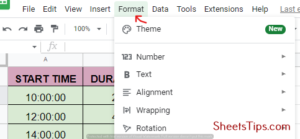
- Step 2: From the drop-down list that opens, scroll the cursor down over the Number option and click on Custom number format.
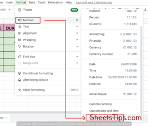
- Step 3: Under the Custom number formats dialog box, type the following format [hh]:mm:ss and click on Apply as shown below:

Thus, the previous steps will format the cells to show us the hours even if the total is exceeding 24 hours.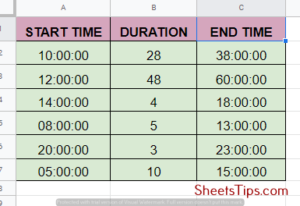
How To Convert Time to Number in Google Sheets?
If you want to convert time to a number or decimal format, then you can achieve this either by using the Time Functions of HOURS, MINUTES, and SECONDS from Google Sheets or by performing simple multiplication with the TIMEVALUE function. Let’s see how to use the time functions in Google Sheets first. As already discussed above, the functions look like = HOURS (time), = MINUTES (time) and = SECONDS (time) respectively.
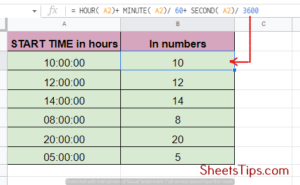
In order to convert the time to the decimal equivalent of the total number of hours, let’s say we have the below mentioned table. Next, use the formula = HOUR( A2)+ MINUTE( A2)/ 60+ SECOND( A2)/ 3600. This formula individually converts minutes and seconds to hours by dividing with 60 and 3600 respectively and then adds it to the hour’s column to generate a total value.
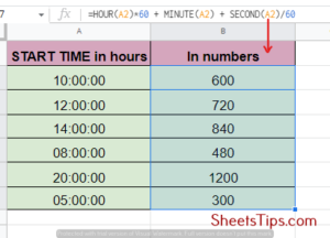
Next, to convert the time to the decimal equivalent of the total number of minutes, use the formula =HOUR(A2)*60 + MINUTE(A2) + SECOND(A2)/60. This formula will individually convert hours and seconds to minutes by multiplying and dividing them by 60, respectively, and then add the value to the minutes column to generate a total answer.
Finally, if we want to convert the time to the decimal equivalent of the total number of seconds, use = HOUR( A2) * 3600 + MINUTE( A2) * 60 + SECOND( A2). This will individually convert the hours and minutes to corresponding seconds by multiplying them by 3600 and 60 respectively and then add the final value to the second’s column to generate a whole answer.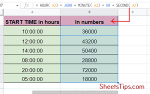
How To Add Time Tracker in Google Sheets?
Tracking time on Google Sheets is simple and comes with many options. You can either track it personally by doing time entries manually or use dedicated formulas for the same. Let’s see the steps to manually tracking time first:
- Step 1: First, select the cells that include the start and end time, then click on the 123 button from the menu bar to select the time option.
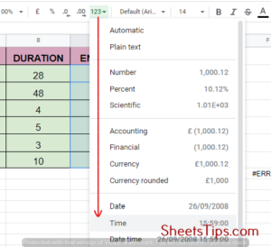
- Step 2: Format the Time menu to Duration and enter the value B2-A2 as shown in the example below to enter the hours worked. Next, drag the fill handle plus button down to apply the formula throughout the column.
![]()
Now, let us take some situations as references and see what formula we can use to track time during them:
- To create a break start and break end, the first format both the column heads to time format by clicking on the 123 buttons as mentioned above. Next, use the formula (B2-A2) + (D2-C2) to calculate the hours worked.
- Shortest and the longest amount of time worked: To get the shortest duration of work done, click on the cell where you wish to display the output and apply the formula =MIN( hours worked column) or =MIN( E: E ) as per the following example. To get the maximum amount of work done, use the formula =MAX( hours worked column).
- Finally, to calculate the total number of hours worked, simply click on the result cell reference again and provide the formula =SUM( hours worked column).
Also, you can access timesheets in Google Sheets to get a template for time tracking. The timesheets you get here are daily, weekly, bi-weekly, and m
