
Copy Conditional Formatting in Google Sheets: If you are somebody who has worked or still works with Google Sheets to handle company or employee data, then you must be fond of formatting cells differently based on various criteria for making the sheet more interesting and understandable. So, have you also wondered how to copy and paste the conditional formatting in Google Sheets?
Well, conditional formatting is an amazing tool to highlight cells based on their value. This helps in making the data more readable and meaningful. In this article, we will teach you how to use conditional formatting in Google Sheets for the same or different sheets and workbooks. So stay tuned till the end if you want to know about these amazing Google Sheet tips.
- How to Conditional Formatting in Google Sheets?
- How to Copy Conditional Formatting to Other Cells in Google Sheets?
- How to Copy Conditional Formatting to Another Sheet?
- Copy Conditional Formatting to Another Workbook in Google Sheets
- How to Do Duplicate Conditional Formatting in Google Sheets?
- How to Copy Conditional Formatting With Relative Cell References?
- Google Sheets Conditional Formatting Based on Another Cell Value
- How to Copy Conditional Formatting in Google Sheets by Expanding the Cell Range?
- FAQs on Copy Conditional Formatting in Google Sheets
Conditional Formatting in Google Sheets
As we all have learned, conditional formatting helps us highlight a range of cells based on certain conditions rather than going to each cell and setting its format. Let’s see the steps we need to follow here:
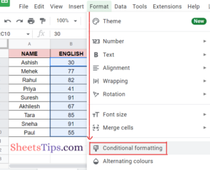
- Step 1: First, select the cell or range of cells where you want to apply format rules and then click on Format from the tools bar, followed by Conditional formatting.
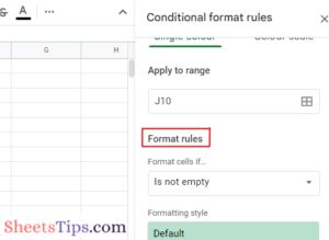
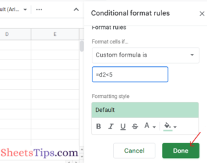
- Step 2: Next, from the Conditional formatting side bar that opens, create a rule depending upon your goals:
- For single color, select the condition that you want to trigger the rule under the Format cells if option and select what the cell will look like when conditions are satisfied below the Formatting style menu.
- Select the color scale of your choice under Preview and select the minimum and maximum value along with an optional midpoint value.
Step 3: Finally, click on Done.
How To Copy Conditional Formatting To Other Cells in Google Sheets?
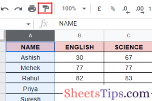
Let us consider the following table as an example here. The table below shows the names of students along with their scores in English and Science, respectively. Now, we applied conditional formatting in column B to highlight the names of the students who have failed and scored less than 40. Let’s see the various options and their detailed steps to copy this conditional formatting to the column C for Science as well: 1. Using the Paint Format Tool—This tool is similar to the MS Excel Format Painter tool. This tool helps you copy the format from one cell and paste it to another cell or range of cells. Let’s see the steps:
- Step 1- Take your cursor and select the particular cell or range of cells from where you wish to copy the conditional formatting, and click on the Paint Format tool from the toolbar.
- Step 2- Next, take your mouse again and click on the cell or range of cells to which you want to apply the copied format.
 One thing one can see here is that the Paint Format tool cannot be used multiple times, unlike the Format Painter of Google Sheets. You will always have to go back and select the new cell range followed by activating the Pain Format tool every single time. Also, you will not be able to use this tool to copy the conditional formatting to a different sheet. 2. Using Paste Special-Paste Special is yet another popular tool to copy the conditional formatting to different cells. Let’s see the steps now:
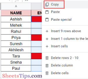
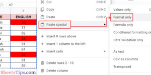
- Step 1: As usual, select the cell or range of cells from which you want to copy the conditional format, right-click, and click on Copy, or you can also press the combination Ctrl+C on your keyboard.
- Step 2: Next, select the next cell or range of cells where you want to paste the format and right-click.
- Step 3: From the drop-down menu, select “Paste Special” and click on “Paste Format Only. The Google Sheets’ conditional formatting shortcut is Ctrl+ Alt+ V, so you can use that too.
 You can use the Paste Special tool on a different sheet from the same document as well. One thing to note here is that using Paste Special to a different range of cells in the same sheet will not create any new rules. Instead, it will extend the new cell range under the same Conditional Formatting rule only. But for cells from different sheets, it will require new rules as per criteria.
How To Copy Conditional Formatting to Another Sheet?
Let’s quickly take the following example as our reference and see the steps to copy the conditional format from one sheet to another: Step 1: First, right-click on the first sheet tab from where you wish to copy the format, select Copy to, and finally click on Existing Spreadsheet.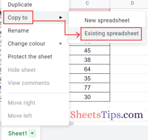 Step 2: Next, from the dialogue that opens, select the file where you want to paste this format, or directly paste the URL on the sheet if it is open, and click on Select.
Google Sheets: Copy Conditional Formatting to Another Workbook
We can easily use the Paint Format tool to copy the conditional formatting from one range to another workbook in Google Sheets. Let’s see the steps to do it:
- Step 1: Select the range of cells you want to copy the format from and click on the Format Painter tool from the upper Tools bar.
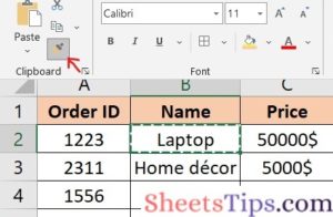
- Step 2: Open your second workbook, select the destination range of cells into which you want to paste the format, and drag the Format Painter tool across the range.
- Step 3: Next, click on the Home button, select Conditional Formatting, followed by Manage rules.
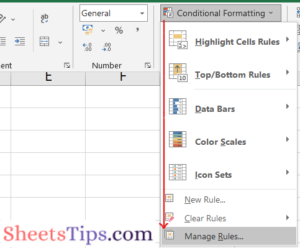
- Step 4: Double-click on the ruler that does not work with the destination range in the Conditional Formatting Rules Manager dialogue box.
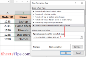
- Step 5: In the Format values where this formula is true box, enter the destination range cell reference and change the formula to =COUNTIF ($B$23: $B$46, $B23) > 1, where $B$23: $B$46 is the second column and $B$23 is the first cell of the destination range. Finally, click on OK to save the changes.
How To Do Duplicate Conditional Formatting in Google Sheets?
Sometimes, you may want to apply the same conditional formatting to a sheet but with a different rule. Yes, Google Sheets does allow you to set the same condition for a range of cells but adjust the formatting accordingly, with the help of the duplicating rule method. Let’s take an example to understand this better and see the steps to do the same:
- Step 1: First, select the range of cells and go to Format from the tools bar, followed by the Conditional Formatting option.
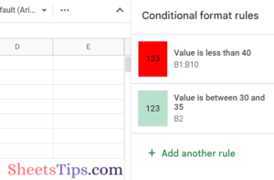
- Step 2: Next, when the sidebar for Conditional Formatting opens, select Add another rule and click on Done thereafter.
 This will duplicate the rule and take you to the main Conditional Formatting screen on the side of the screen. Here, you will be able to see your original rule and its duplicate.
- Step 3: Select the duplicate rule, make your necessary changes based on cell range, conditions, and formatting, and finally click on Donewhen you are finished with it.
How To Copy Conditional Formatting With Relative Cell References?
Relative cell referencing provides us with the provision of applying a single conditional format formula to an entire row or column range of cells, in the same sheet or different. Let’s see what the steps are separately for column and row cell ranges: For Column Range: From the example given below, let’s assume we want to format the values in A2:A if B2:B is pending. For this, first, go to the Format option from the tools bar and select Conditional Formatting. Then, from Format Rules, select Custom Formula and insert the syntax =B2=”Pending” or =$B2=”Pending”. Next, insert A2:A in the Apply to range field inside the Conditional Format Rule panel. 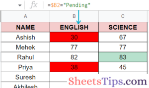 For Row Range: This is completely similar to the formulas above, just make sure you put in the row ranges correctly. So here, in the Apply to range field, put B1: K1. Next, change the range to highlight from A1: K1 to A1: K2 and apply the formula =B$2=” Pending”. For copying formats to different sheets, you will need to use the INDIRECT function. The formulas now for the row range will be =indirect(“‘Sheet2’!” &address( row( B)), column(B2), 4))=”Pending” and for the column range will be =indirect(“‘Sheet2’! “&address( row( B2), column( B2), 4))=”Pending”.
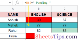
Google Sheets: Conditional Formatting Based on Another Cell Value
Rather than copying the conditional formatting rules from one parent cell to the other, you can also copy conditional formatting based on another cell value. Let’s see the steps for the same:
- Step 1: Select the cell or cell range you want to format and click on Format from the navigation tools bar, followed by clicking on Conditional Formatting.
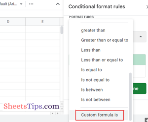
- Step 2: Next, when the sidebar for Conditional Formatting opens, select Custom formula under Format rules.
- Step 3: After adding the formula based on your choice click Done and confirm the other cell’s range under Apply to range.
How To Copy Conditional Formatting in Google Sheets by Expanding the Cell Range?
Well, no one wants to follow lengthy steps while in a hurry. So, in case you are wondering whether you always need to follow the detailed steps mentioned above to copy the conditional formatting to cells, then no, you can also do this by editing a rule and simply expanding the range of cells on the same. Let’s see the steps now:
- Step 1: Select the cells, click on Format from the toolbar above, and select Conditional formatting.
- Step 2: From the Conditional Formatting sidebar that opens, select the rule you want to copy and click on the Grid box to add the new cell range you want to expand it with.
- Step 3: Next, from the Select a data range box, below the first range, input the second range of cells you want to highlight to automatically select the range for the given rule.

- Step 4: Finally, in the data range box, click Ok, and in the conditional formatting box, click Done.
FAQs on Copy Conditional Formatting
1. Can you copy conditional formatting in Google Sheets?
Yes, of course. You can use tools, namely Paint Format and Paste Special, to copy conditional formatting from one cell to another cell, or a range of cells within the same sheet or different.