
Google Sheets VLOOKUP function is one of the classy functions which helps to find a value or an item in a table or a row and returns it. But one of the major drawbacks with the VLOOKUP function is that we cannot VLOOKUP in the opposite direction i.e., VLOOKUP Left is impossible.
However, with the help of sneaky tricks, we can simply perform a reverse VLOOKUP right to left in Google Sheets. So why wait? Read further to know how to perform the VLOOKUP Left function using the Google Sheets Tips provided on this page.
Table of Contents |
How Do You VLOOKUP The Opposite Direction in Google Sheets?
In order to enable the VLOOKUP function to work in an opposite direction, firstly we will have to create a virtual table. The virtual table must be created in such a way that the columns are switched in reverse order.
- How to VLOOKUP from Another Sheet in Google Sheets: Vlookup Between Two Sheets
- How to Use IMPORTDATA function in Google Sheets? (Fetch CSV/TSV File)
- How to Analyze Data from Google Sheets with Examples
How To VLOOKUP To The Left in Google Sheets?
Consider the table in the following image where you want to perform the VLOOKUP Left. Now the steps to perform the VLOOKUP left is as follows:
- 1st Step: Open the Google Spreadsheet where you want to perform the VLOOKUP left.
- 2nd Step: Now in this example, we have a table and now we need to create a virtual table.
- 3rd Step: Move to the cell where you want to create a virtual table. The array formula to create a virtual table is ={B1:B10,A1:A10}.
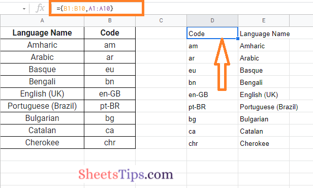
- 4th Step: Press the “Enter” button and the virtual table has been created in the Google Sheets. Curly brackets signify an array in this formula, and the two columns are switched within. This produces an array with the two columns reversed.
- 5th Step: Now we need to alter the array virtual table formula with the VLOOKUP function. The modified formula is =VLOOKUP(D2,{$B$1:$B$10,$A$1:$A$10},2,FALSE).
- 6th Step: Now use this formula and press the “Enter” button.
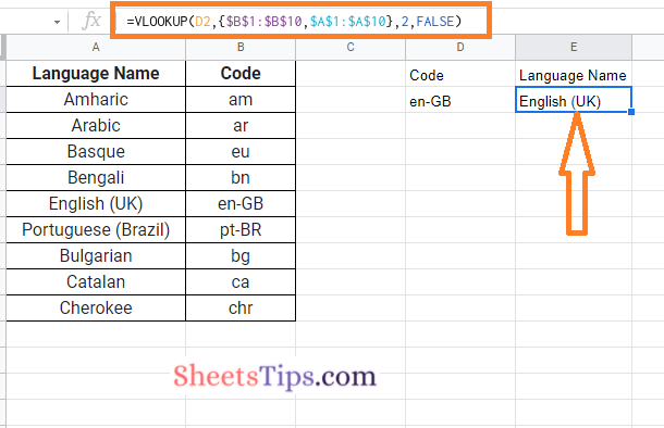
That’s it. The VLOOKUP left function has been executed in the Google Sheets. This method is much easier when compared to INDEX and MATCH functions in Google Sheets.