A technique where we apply chain rule multiple times is known as Onion Method. This technique is called as Onion method since we perform one action per one step which is more or less like peeling the Onion. This Onion method comes in handy when we build complex formulas in Google Sheets. If you are unaware of how to adapt the Onion method to build complex formulas in Google Sheets, then this will tell you everything about it. Using the Google Sheets Tips and Tricks provided on this page, we can easily build complex problems in a spreadsheet.
Table of Contents |

How To Build Onion Method for Complex Formulas?
To build an onion method for complex formulas, we will have to follow the one action per step approach. This means we will have to build our formulas in a series of steps.
Confused about how to do this? Well, don’t worry. We have outlined how to build formulas using the Onion Framework here.
Onion Framework consists of three important elements and they are outlined below:
- Firstly outline the step-by-step formula that you will be using in your Google Sheets and put each formula in each of the cells.
- Now label the formulas with the step number in the adjacent cell. For example, if you want to use the IF function formula in the third step, you can simply name it Step 3.
- Then enable the different background colors against each formula cell to make it more identical.
This allows you to observe the formula move in a step-by-step manner, which is extremely useful when creating or trying to grasp complex formulas in Google Sheets.
- How to Get Running Totals in Google Sheets (Easy Formula)
- Google Sheets QUERY Function Explained With Examples
- How To Use Sequence Function To Build Numbered List In Google Sheets?
Example: Build Complex Formulas in Google Sheets using Onion Method
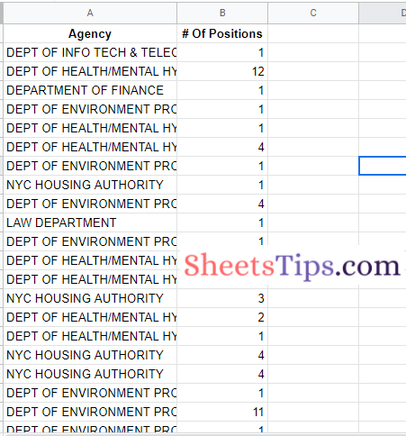
Let us consider the following example where we have the organization’s name and list of available positions. If you see the dataset, it is unorganized.
We can organize this dataset with the help of complex formulas using the Onion framework and summarise the job openings. The steps to get this done are outlined below.
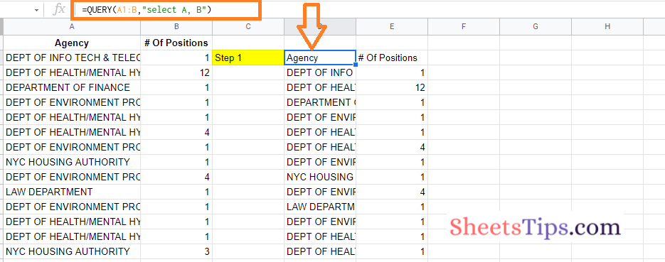
Step 1:
Firstly let us use the Query function to summarise the data. Since we have two columns – A, B, we will select these two columns using the Query function. The formula to select these two columns using the Query function is as follows:
=QUERY(A1:B,”select A, B”)
Although this has no effect on the data, it’s usually a good idea to run a simple query first to confirm you’re using the proper dataset as the input to your QUERY function.
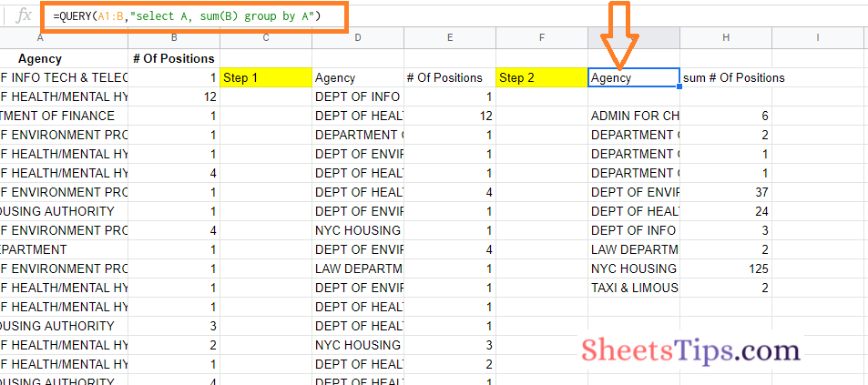
Step 2:
Now we are supposed to summarise the job position in Google Sheets using the GROUP BY clause. We are using the GROUP BY clause inside the QUERY function. The formula to get this done is Google Sheets is as follows:
=QUERY(A1:B,”select A, sum(B) group by A”)
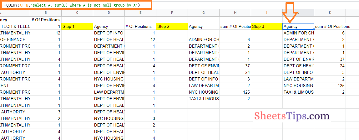
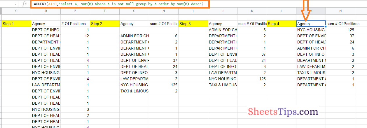
Step 3:
Now the next step is to filter out the blank rows. To do this, we will have to use the WHERE clause. This WHERE clause will be used inside the query function and GROUP BY clause as shown below:
=QUERY(A1:B,”select A, sum(B) where A is not null group by A”)
Step 4:
Now the next step is to use the ORDER BY clause. The ORDER BY clause is used here to sort the selected dataset in descending order. So our formula in the 4th step will be as follows:
=QUERY(A1:B,”select A, sum(B) where A is not null group by A order by sum(B) desc”)
Step 5:
In this step, we will have to fix the header of the total column using the LABEL clause. The formula to be used in this step is as follows:
=QUERY(A1:B,”select A, sum(B) where A is not null group by A order by sum(B) desc label sum(B) ‘Total Positions'”)
Press the Return key after using this formula in Google Sheets and you will see the results being generated as shown in the image below.
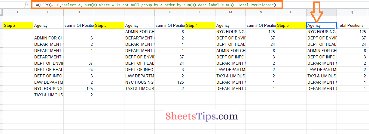
Rather than utilizing a pivot table, we used the QUERY function to generate one. The key to making this work was to build it in steps, with the formula changing slightly with each step.
Step 6:
In this step, we are using the array literals. For this, we need to add a placeholder line in the total row and the formula for the same is as follows:
={QUERY(A1:B,”select A, sum(B) where A is not null group by A order by sum(B) desc label sum(B) ‘Total Positions'”);{“TOTAL”,”TBC”}}
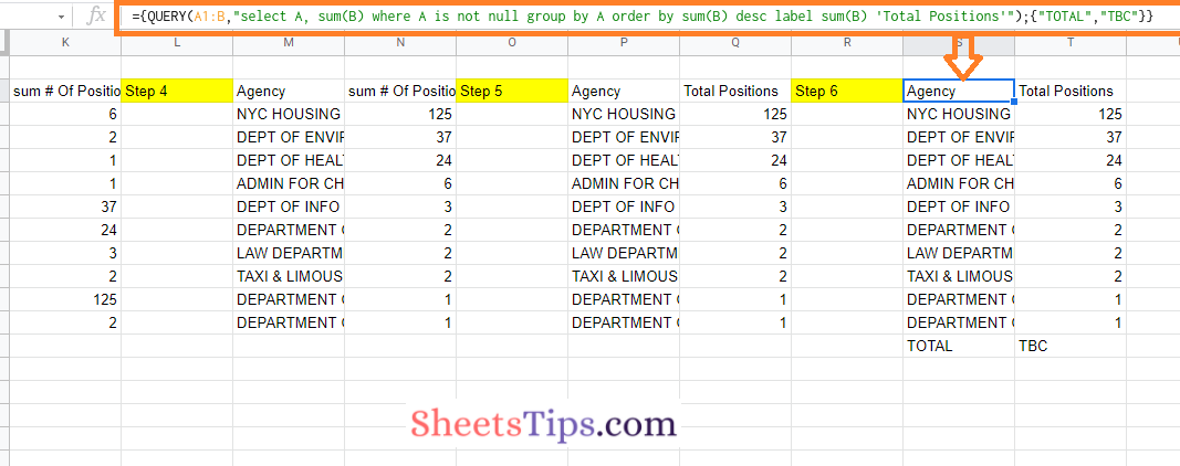
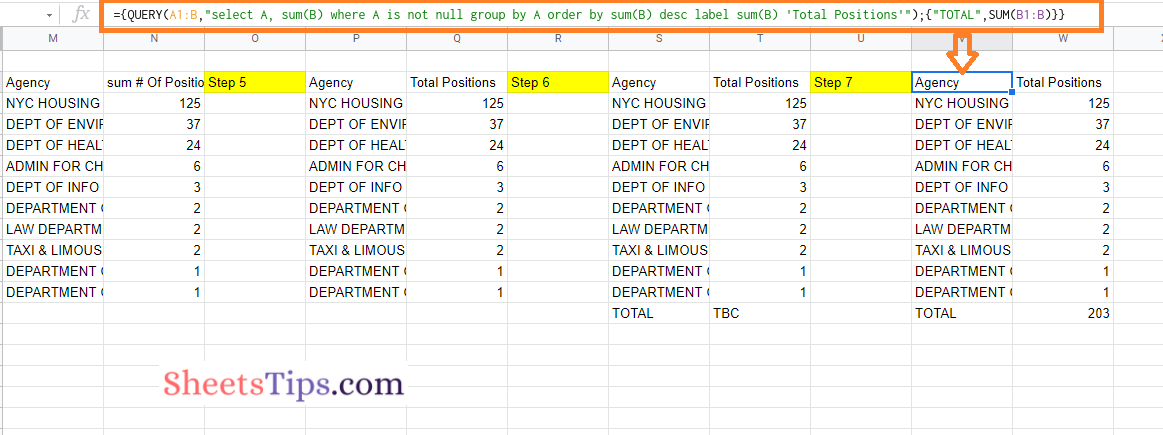
Step 7:
To get the right total, we need to convert this placeholder into an actual formula. We leave the range reference open-ended, much as the data provided to the query function, to guarantee that it remains dynamic and will automatically incorporate fresh data. So our formula in this step will be as follows:
={QUERY(A1:B,”select A, sum(B) where A is not null group by A order by sum(B) desc label sum(B) ‘Total Positions'”);{“TOTAL”,SUM(B1:B)}}
Now that you will have an idea of how to build complex formulas in Google Sheets using the Onion Method Framework. If you are attempting to figure out complicated formulae in Google Sheets that someone else has provided with you, you can still use the Onion Method.
Simply peel back the layers until the deepest function is disclosed. Copy the formula into a new cell and work your way up to the whole formula again, starting from the inside.