
A Simple Guide to Hide Columns in Google Sheets: Sometimes, while handling certain spreadsheets, we may encounter situations in which we need to hide certain columns or rows but not delete them completely. In this article, we will show you how to hide and lock columns and rows that are not useful or private to certain users, both for basic and advanced levels of data handling in Google Sheets.
Also Read: Python: Add a Column to an Existing CSV File
So let’s quickly brush up our knowledge on how to hide and unhide columns in Google Sheets and make sure to stay tuned till the end to learn the most about these amazing Google Sheet tips for rows and columns.
- How To Remove Columns in Google Sheets?
- Shortcut To Hide Columns in Google Sheets
- How To Hide Unused Columns in Google Sheets?
- How To Hide and Lock Columns in Google Sheets?
- Google Sheets Hide Columns Based on Cell Value
- Steps To Show Hidden Columns in Google Sheets
- How To Hide Rows in Google Sheets?
- How To Hide Rows in Google Sheets Without a Right Click?
- FAQs on Hiding Columns
How To Remove Columns in Google Sheets?
If you wish to remove a column totally from a certain table on Google Sheets, then follow the steps given below:
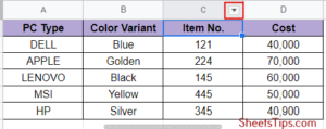
Step 1: First, left-click on the column you wish to delete or remove from the table. Next, go to the column head and click on the small down arrow key button next to it.
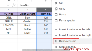
Step 2: Here, you will see a drop-down list open. Click on Delete Column to permanently remove the column from the table.
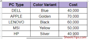
Step 3: Now, you will see your table being displayed without that particular column. Without removing the whole column, if you wish to just clear the contents to refill them, then you can click on Clear Column.
How To Hide Multiple Columns in Google Sheets?
To hide multiple columns or rows from a Google Sheets table, you need to follow the steps given below:
Step 1: First, click on the first row/column from which you want to hide and then drag it to the last row/column from which you want to hide. You can also press the Shift key and click on the last row or column you want to hide.
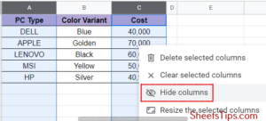
Step 2: Right-click here and from the drop-down list, select the option Hide rows/columns n-n, which indicates the selected rows/columns you wish to hide.
Step 3: If the rows or columns you want to hide are not contiguous, simply hold down the Ctrl key and left-click on the rows or columns you want to hide.
Step 4: Finally, right-click on any of the rows and select Hide Columns/ Rows from the drop-down list that appears.
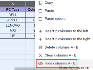
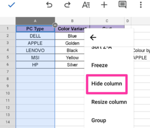
In case you are wondering about how to hide columns in Google Sheets on iPad, simply open the Google Sheets app on your iPad first and long press on the header letter of the column you want to hide. You will see the bar for cut, copy, and paste. Click on the perpendicular three-dot button against it. Select Hide columns from the drop-down list, and you are done.
Shortcut To Hide Columns in Google Sheets
Who doesn’t want shortcuts in his life?!
Well then, let’s see a quick method of hiding columns in Google Sheets by a shortcut. If you are a keyboard person, then this is going to be your go-to. Simply select the columns or range of columns and press CTRL+ALT+0 altogether. Immediately, you will see the selected rows have disappeared from your Google Sheets table. To undo this action, you need to press Ctrl + Z together.
How To Hide Unused Columns in Google Sheets?
While filling out a table spreadsheet on Google Sheets, you may see that some rows and columns have been left unused, so you may wonder how to hide them. Below are the steps that are going to help you with that:
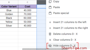
- Step 1: Left-click on the column header and select the first column that is just next to the last used column.
- Step 2: Next, press the Ctrl and Shift keys along with the right-arrow key. This will help you select all the rest of the unused columns.
- Step 3:Finally, right-click on any of the selected portions and select the Hide Columns n-Xoption, where n is the first unused column and Z is the last one.
How To Hide and Lock Columns in Google Sheets?
If you are using Google Sheets as a public medium for your profession, then you might face situations that will make you wonder how to hide columns in Google Sheets for certain users. So, let’s see the steps to protect your columns:
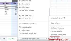
- Step 1: Our first aim is to change the edit permissions. For this, first select the column headers you wish to hide and protect.
- Step 2: Next, right-click on your selection, scroll down to view more column options, and click on Protect range from the drop-down list. This will open the Protect Sheets and Ranges side menu on the right part of the screen.
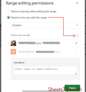
- Step 3: Click on the Range tab followed by the Set permissions button and this will open the Range editing permissions window.
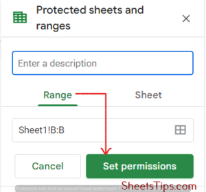
- Step 4: Click on “Restrict who can edit this range. Check the users you want to give access and uncheck the users you want to lock the columns for. Click on Done thereafter.
- Step 5: Now, we can go ahead and hide the columns we want by right-clicking on the selected rows followed by the Hide columns option. The restricted users will not be able to unhide these columns anymore.
Google Sheets Hide Columns Based on Cell Value
The filter option in Google Sheets is basically used to sort and extract elements according to our choice by selecting a filter. Hence, if you want to hide certain columns based on some given cell values in Google Sheets, then the Google Sheets: Filter view – Hide Columns is going to help you. Here are the steps:
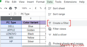
- Step 1: Select the columns you wish to hide and click on Data from the Sheet settings top bar, followed by clicking on the Create a filter option. This will add filters to your selected columns.
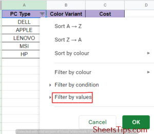
- Step 2: Now, click on the filter buttons of each of the selected columns and click on Filter by values. Now, add the filters and press OK. This will display all the records pertaining to those values.
- Step 3: Select these records and hide them by right-clicking and selecting Hide columns. Again, change the filter to select all and you will be displayed with the new updated table.
Steps To Show Hidden Columns in Google Sheets
Sometimes it may happen that you have mistakenly hidden a column or row and wish to make it visible again to check for its content. Unhiding or making hidden columns visible on Google Sheets is very simple. Simply click on the two arrow buttons in between the columns, within which lies the hidden column.
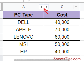
For example, if you have hidden column B, click on the double arrow button between columns A and C. One thing to note here is that you must have edit permission if you wish to access and unhide such columns of a public spreadsheet.
How To Hide Rows in Google Sheets?
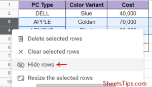
Hiding rows in Google Sheets is quite similar to hiding columns. Simply select the rows you wish to hide by pressing Shift and clicking the two row extremities, or pressing Ctrl and clicking the selected rows if they are not contiguous. Then right-click on the selected portion and click on Hide rows to hide them, where n represents the cell range points.
How To Hide Rows in Google Sheets Without Right Click?
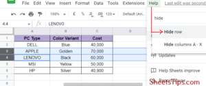
If you wish to hide certain rows in your Google Sheets table without using the right click, then you will have to use the Help section. Let’s see the steps for it:
- Step 1: Select and highlight all of the rows you want to hide.
- Step 2: Next, click on the Help option from the Sheet settings bar and type “Hide” in the Search menu bar.
- Step 3: Finally, click Hide rows n-n to hide your selected rows without having to use your mouse’s right-click button.
FAQs on Hiding Rows and Columns in Google Sheets
1. Why can’t I hide a column in Google Sheets?
You are unable to hide columns or make other changes in Google Sheets, probably because you don’t have permission to edit them. Try contacting the sheet admin to remove your name from restrictions and give you access to make changes.
2. How do I hide and lock columns in Google Sheets?
To hide and lock columns, follow this: select columns to hide< Protect range< Protect sheets and ranges side menu< range tab< set permissions< range editing permissions window< restrict who can edit this range< uncheck users you want to lock< done. Then hide the columns by selecting the columns and pressing CTRL+ALT+0.
3. How do I hide columns in the Google Sheets app?
To hide columns in the Google Sheet app, long press the column header, tap on the three-dot option, and select hide column.