
Google Sheets Compare Data in Two Sheets: We all enjoy comparing things to buy, try, decide, etc., just to get a side-by-side view of the key features of everything. But, did you know you could do that with Google Sheets too? Smaller sheets are easier to work with, but for larger volumes of data, Google Sheets does provide you with certain tools to help you extract minute discrepancies that are impossible for the human eye.
Since Google Sheets doesn’t provide you with any direct function to tackle this, we need to use the in-built tools with a little bit of creativity. In this article, we will discuss all of these Google Sheet tips in detail. Without wasting any more time, let’s roll.
- Compare Two Sheets for Duplicates
- How To Find the Difference Between Two Sheets in Google Sheets?
- Compare Data in Two Sheets To Find Missing Data
- Compare Data in Two Sheets for Exact Row Match
- How To Compare Two Sheets in Google Sheets To Highlight Matching Rows?
- Google Sheets Compare Two Strings
- FAQs
How To Compare Two Google Sheets for Differences?
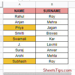
We tend to see a lot of human errors while entering data into Google Sheets. Here, we will learn how to compare two sheets and find out the rows that are exactly repeated in the second sheet. Let’s take the following example as our reference and perform Conditional Formatting to extract and highlight the duplicate data entries in Sheet 2. Here are the steps:
- Step 1: Select the blank column which is just after the right-most column of Sheet 2. We will use column C for this example.
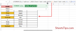
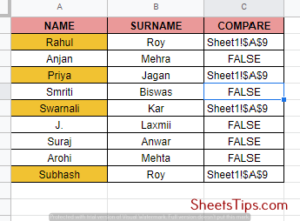
- Step 2: Select the second row of this column and put the formula =IFERROR( CELL( “address”, INDEX (Sheet1! $A $1: $A $9, MATCH( A2, Sheet1! $A $1: $A $9, 0), 1) ), FALSE). This will return the cell address in Sheet 1, Column A that matches exactly with the contents of A2 of our current sheet. The formula will return FALSE if a match isn’t found and both columns are unique.
- Step 3: Now, copy this formula to the rest of the rows of the column by dragging the plus sign fill handle. Now the sheet looks somewhat like this:
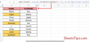
- Step 4: Now we can move forward with our conditional formatting. Follow the steps mentioned in the second last topic of this article, but make sure to input the formula =IF( NOT( C2= FALSE), IF( OFFSET( INDIRECT( C2), 0, 1)= B2, TRUE, FALSE ), FALSE) in the input box of the conditional format rules window.
This will help you highlight all the duplicate column data in Sheet 2 with a single colour for better understanding.
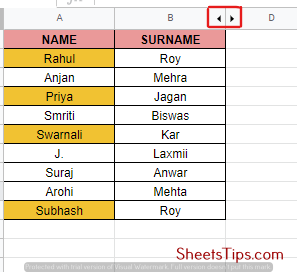
- Step 5: Now, if you are wondering How to compare two columns for unique values in Google Sheets then you can simply hide these duplicates and display the final table. For this, right-click on the columns and click on Hide columns from the menu that appears.
Also read: How to hide columns in Google Sheets?
How To Find the Difference Between Two Sheets in Google Sheets?
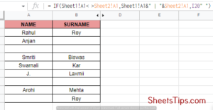
Consider the following scenario: you have two sheets that appear to be identical, but you want to compare them to see if they are identical or have minor differences. Well, you can easily do this by applying a single formula and pasting it through a third sheet. The syntax of this formula is = IF( Sheet1! A1< > Sheet2! A1, Sheet1! A1& ” | ” & Sheet2! A1, ” “), where we have:
- a matching condition
- a text or formula to be returned if the condition satisfies TRUE
- a text or formula to be returned if the condition is FALSE
The condition is that cell A1 of Sheet1 is not equal to cell A1 of Sheet2. If the condition is true, the function will return the value in Sheet1, cell A1, followed by a pipe symbol, and followed by the Sheet2, cell A1 value, i.e, Sheet1! Sheet1 & | & Sheet2!A1.
And, if the condition is false, the function will simply return a blank cell (“”). Once we paste this formula throughout the cells of the third sheet, Sheet3, it is going to display the exact mismatched cells as well as the differences. Let’s see the steps now:
- Step 1: Create the third sheet by clicking on the ‘+’ icon beside Sheet 2. Rename this new tab “Sheet3.”In the cell A1 of Sheet 3, put the formula: =IF( Sheet1! A1 <> Sheet2! A1, Sheet1! A1 &” | “& Sheet2! A1, ” ” )
- Step 2: Copy the formula above to your clipboard.
- Step 3: Next, select all the cells of Sheet 3 by pressing the key combination “Ctrl+A” on your keyboard and pressing “Ctrl+V” from your keyboard to paste this formula throughout all the selected cells of Sheet 3.
How To Compare Data in Two Sheets To Find Missing Data in Google Sheets?
While filling out a data spreadsheet on Google Sheets, we might miss entering certain values. So, if you want to extract and highlight the missing rows instead of the duplicate ones, you just need to highlight the opposite rows.
This will work just by adding a simple NOT function outside the conditional formatting formula.
The syntax to use is =NOT( IF( NOT( C2= FALSE), IF( OFFSET( INDIRECT( C2), 0, 1)= B2, TRUE, FALSE), FALSE )).
How To Compare Data in Two Sheets for Exact Row Match?
Let’s consider comparing the two sheets of ours row-wise and displaying the results on the third sheet, Sheet 3. The output will be matching if the rows match in both the sheets on the corresponding row of Sheet 3 and not matching if they don’t match.
For this, we will need to use an IF function with a nested AND that will have more than one condition as a parameter and will return TRUE if all the conditions are satisfied; False otherwise. The steps to follow are:
- Step 1: Create a third Sheet by clicking on the + button against Sheet 2 at the bottom bar of the window.
- Step 2: Next, in cell A2 of Sheet 3 insert the formula: =IF( AND( Sheet1! A2= Sheet2! A2, Sheet1! B2= Sheet2! B2) ,”Matching”, ”Not Matching”).
- Step 3: Finally, copy this formula down to the rest cells of the column by dragging the + sign fill handle.
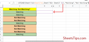
You will now see the output ‘Matching’ wherever the corresponding rows of Sheets 1 and 2 matches, and ‘Not Matching’ else.
How To Compare Two Sheets in Google Sheets To Highlight Matching Rows?
If you want to highlight the matching rows or columns within one of our two sheets rather than displaying all the results on a separate sheet, then you must use the Conditional Formatting feature of Google Sheets. In simple words, conditional formatting is nothing but a technique that helps you format cells depending upon a condition.
Conditional Formatting does not allow us to use cell references from another sheet. So we have to use the INDIRECT function to access the other sheet indirectly.
This formula will compare two columns of each row in Sheet1 and Sheet2 and will use the INDIRECT function to extract a direct cell reference to columns A and B of Sheet1. Next, it will check whether the cells corresponding to both the columns in each row match and highlight the row accordingly.
Here are the steps to do this:
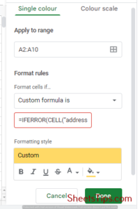
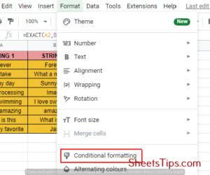
- Step 1: Click on the Format menu from the menu bar and select Conditional Formatting.
- Step 2: When the ‘Conditional format rules’ sidebar opens on the right part of the window go to Apply to range under the input box and insert the cell range you want to apply the Conditional formatting to. In this example, type Sheet2! A2: A10 to apply formatting to Sheet 2.
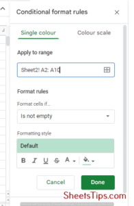
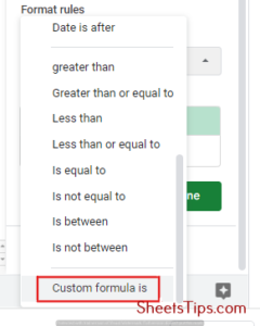
- Step 3: Under the Format rules section, go to the Format cells if section and click on the dropdown arrow to select “Custom formula is” from it.
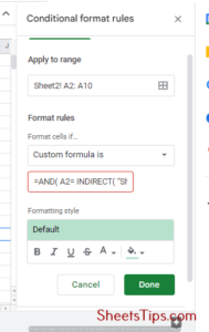
- Step 4: Below the dropdown list go to the input and type the formula =AND( A2= INDIRECT( “Sheet1! A2: A” ), B2= INDIRECT( “Sheet1! B2: B” ) )”.
- Step 5: Under the Formatting style option click on the Fill Color button and select your favorite for highlighting the matching rows.
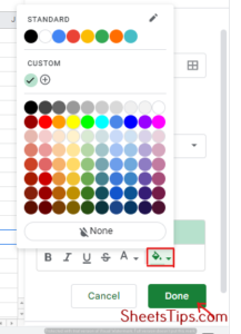
- Step 6: Finally, click on the Done button to save the changes and initiate Conditional formatting. As a result, you will see the matching rows highlighted in the color you chose.
In case your sheets have more than two columns, expand the INDIRECT function by adding more parameters that compare each column.
For 3 columns, your formula would be =AND( A2= INDIRECT( “Sheet1! A2: A”), B2= INDIRECT( “Sheet1! B2: B”), C2= INDIRECT( “Sheet1! C2: C”) )”. Additionally, if you want to highlight only rows that don’t match, just replace the ‘=’ symbols with ‘<>’.
How To Compare Two Strings in Google Sheets?
We all know that strings are a combination of characters that add up to form a meaningful sentence. So, in some cases, you may need to compare any two adjacent cells of strings in any worksheet and mark their differences and similarities. The EXACT function is going to help you here. Let’s understand this better with an example.
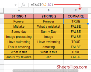
Let’s suppose in the above table you want to compare the two strings in columns A and B, and whether they are matched or not. Simply apply the formula =EXACT(A2, B2) in the blank cell C2 and press Enter. Now select the fill handler key and drag it down to the last cell to apply the formula to the entire result column. The outputs displayed will be TRUE if they match and FALSE if they don’t.
Read Also: Java interview questions