
When you are working with a numerical dataset, it is quite common to experience negative numbers. If your dataset is small, then it’s very easy to identify the negative numbers to understand the detailed analysis of the data. However, if you are working with a large dataset, then manually checking the negative numbers would be difficult. And hence, to help with the problem, Google Sheets allows its users to highlight the negative numbers in the desired color.
For example, let us assume that you are working with November sales data and you want to compare the current sales month data with the previous month’s to know where you have performed well and where you haven’t. If you have 10 rows of data, then you can quickly analyze the results. However, if your dataset is quite large, then manually drawing the conclusion would be difficult. To help you overcome this issue, here is a detailed page that teaches you how to highlight the negative number in red using the Google Sheets Tips. Scroll down to find out more.
| Table of Contents |
How to Make Negative Numbers Red in Google Sheets?
There are various methods with the help of which we can highlight the negative numbers in red. One of the easiest methods to highlight the negative numbers in red is by using the Custom number format. The detailed steps on how to change negative numbers into red using the custom number format are explained below.
- 1st Step: First, launch Google Sheets on your device.
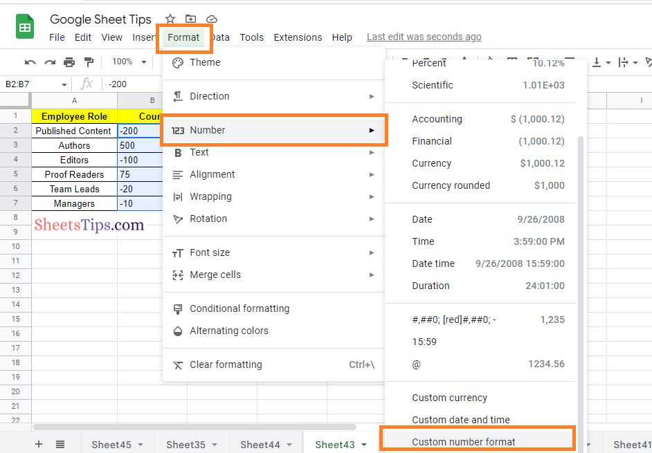
- 2nd Step: Select the dataset and click on the “Format” tab.
- 3rd Step: Choose “Number” and select “Custom number format” towards the bottom of the drop-down list.
- 4th Step: Now paste the formula “#,##0; [Red](#,##0)” in the Custom number format box.
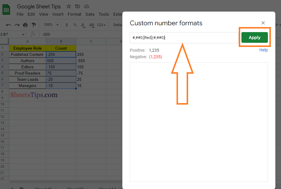
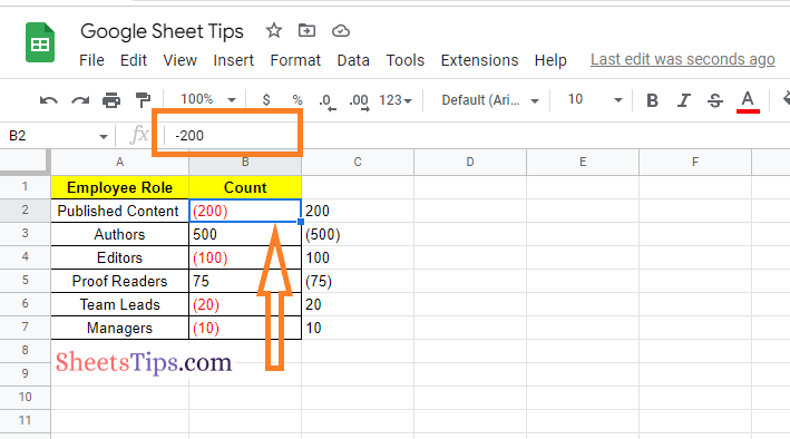
- 5th Step: Press the “Apply” button and you will see the negative numbers being highlighted in red.
Apart from the above formula, one can also use the following formulas in the Custom number format box to get the same results:
- #,##0;[Red]#,##0
- #,##0;-[red]#,##0
Using Conditional Formatting To Show Negative Numbers As Red in Google Sheets
Google Sheets also allows its users to change the negative numbers into red using the Conditional Formatting option. The detailed steps on how to get this done in the spreadsheet are outlined below:
- 1st Step: Open the Google Spreadsheet on your device.
- 2nd Step: Now on the homepage, select the dataset which needs to be highlighted in red.
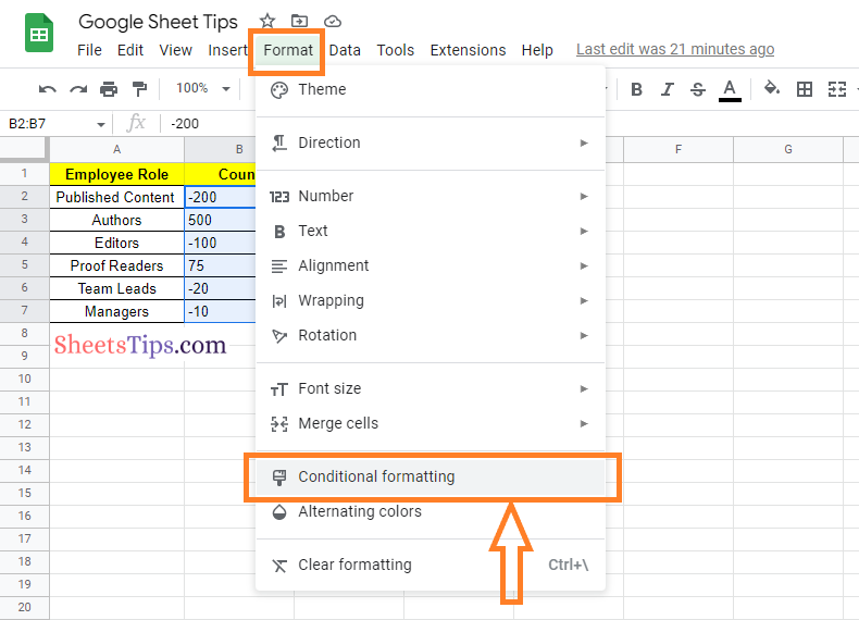
- 3rd Step: Click on the “Format” tab and choose “Conditional Formatting” from the drop-down menu.
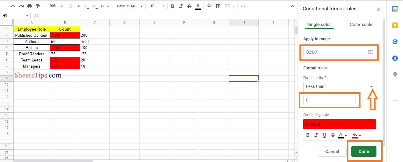
- 4th Step: The Conditional Formatting menu opens on the screen. Now cross-check the cell range under the “Apply to Cell Range” box.
- 5th Step: Under the “Format Rules” tab, choose the “Less than” option.
- 6th Step: In the “Value or Formula” box, enter the number Zero.
- 7th Step: In the “Formatting Style“, click on the Text Color and choose the color “Red” to highlight the data in red. If you also want to highlight the cell in red, then choose “Red” color from the Fill Color.
- 8th Step: Press the “Done” button and you will see the results as shown in the image given below.
Using Apps Scripts to Change Negative Numbers to Red
Apart from the above-listed steps, one can also use Apps Scripts to highlight the negative numbers in red. The steps to do this in the Google Sheets are given below:
- 1st Step: First, launch Google Sheets on your device.
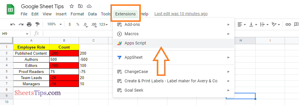
- 2nd Step: Now on the homepage, click on “Extensions” and choose “Apps Scripts” from the drop down menu.
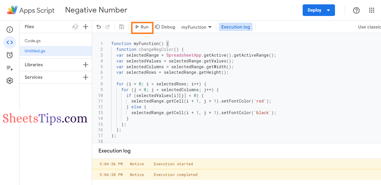
- 3rd Step: Here we are creating a function called “ChangeNegColor“. Once you open the Apps Script code editor, paste the code which is tabulated below:
function changeNegColor() { var selectedRange = SpreadsheetApp.getActive().getActiveRange(); var selectedValues = selectedRange.getValues(); var selectedColumns = selectedRange.getWidth(); var selectedRows = selectedRange.getHeight(); for (i = 0; i < selectedRows; i++) { for (j = 0; j < selectedColumns; j++) { if (selectedValues[i][j] < 0) { selectedRange.getCell(i + 1, j + 1).setFontColor(‘red’); } else { selectedRange.getCell(i + 1, j + 1).setFontColor(‘black’); } }; }; }; function onOpen() { var ui = SpreadsheetApp.getUi(); ui.createMenu(‘Negatives’) .addItem(‘Change Negative to Red’, ‘changeNegColor’) .addToUi(); }; |
- 4th Step: Click on the “Save” button and “Run” the code.
- 5th Step: Return to Google Sheets and refresh the sheet.
- 6th Step: In the menubar, click on the “Negatives” and choose “Change Negative to Red” from the drop down.
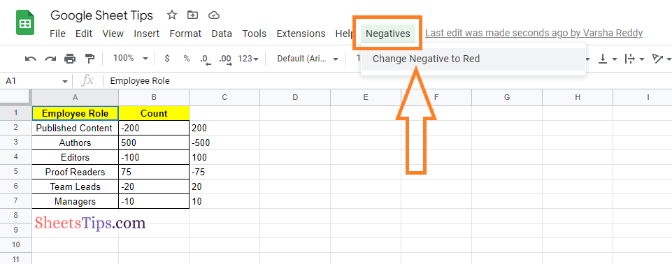
The above steps will change the color of negative numbers to red. The script used here will loop into all the cells and change the font color to zero if the number or value is less than zero.
Now that you have provided all the necessary information on how to change the negative number value to red in the Google Sheets. With the help of the above three methods, choose the one that fits your dataset the best.