Subtotal Function Syntax in Google Sheets
The syntax of Google Sheets’ Subtotal function is as follows:
- Function_Code: The function code here specifies the function to be used in subtotal aggregation.
- Range 1: This specifies Range 1 for which the subtotal needs to be calculated.
- Range 2: Additional ranges which we can specify to calculate the subtotals.
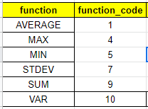
| Function | Code (includes hidden values) | Code (ignores hidden values) | Function Code Meaning |
| AVERAGE | 1 | 101 | The AVERAGE function returns the numerical average value in a dataset, ignoring the text. |
| COUNT | 2 | 102 | Returns the number of numeric values in a dataset. |
| COUNTA | 3 | 103 | Returns the number of values in a dataset. |
| MAX | 4 | 104 | Returns the maximum value in a numeric dataset. |
| MIN | 5 | 105 | Returns the minimum value in a numeric dataset. |
| PRODUCT | 6 | 106 | Returns the result of multiplying a series of numbers together. |
| STDEV | 7 | 107 | The STDEV function calculates the standard deviation based on a sample. |
| STDEVP | 8 | 108 | Calculates the standard deviation based on an entire population. |
| SUM | 9 | 109 | Returns the sum of a series of numbers and/or cells. |
| VAR | 10 | 110 | Calculates the variance based on a sample. |
| VARP | 11 | 111 | Calculates the variance based on an entire population. |
How to Use the Subtotal Function in Google Sheets?
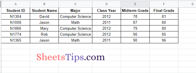
Let us understand more about the Subtotal function in Google Spreadsheet using an example. Consider the following dataset where we have student grade reports:
| Student ID | Student Name | Major | Class Year | Midterm Grade | Final Grade |
| N1304 | David | Computer Science | 2012 | 78 | 81 |
| N1008 | Jason | Math | 2011 | 87 | 80 |
| N1866 | Mary | Computer Science | 2012 | 79 | 80 |
| N1774 | Rob | Computer Science | 2012 | 90 | 85 |
| N1365 | Jason | Math | 2011 | 90 | 96 |
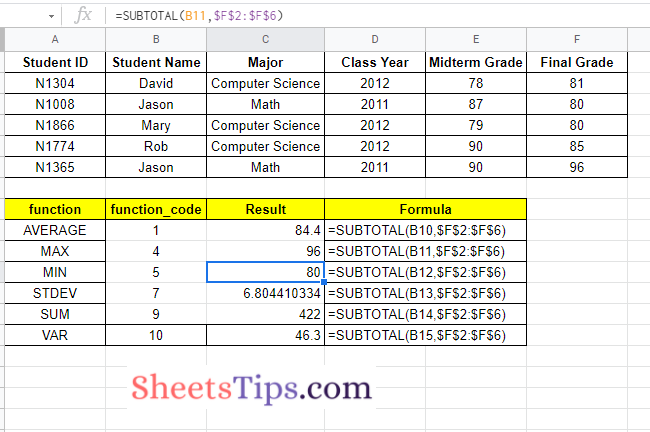
Now let us perform a few subtotal functions such as AVG, Max, Min, STDEV, SUM, and VAR with the students’ grade reports. The steps to get this done in Google Sheets are as follows:
- 1st Step: Open the Google Spreadsheet on your device.
- 2nd Step: Now copy-paste the student grade report for which you want to perform the subtotal function.
- 3rd Step: Next, move to the cell where you want to perform the subtotal function. Here I am creating a dataset for the calculation of subtotals, as shown in the image below.
- 4th Step: Now in the “Result” column, enter the formula as =SUBTOTAL (B10, $F$2: $F$6).
- 5th Step: Press the “Return” key and you will see the results as follows.
- 6th Step: Now drag the formula-applied cells to other cell ranges and you will see the subtotals being calculated as shown below.
How to Create a Subtotal Function for Hidden or Filtered Data?
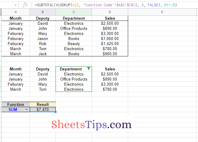
Let’s say we have a huge data collection that has been classified and filtered by the department. To review the data in our reports, we have total cells. The purpose is to have the total cells adjusted as an outcome of the filter. So, if we’re looking at data about electronics, the total number of cells must reflect that.
Also, if a row is hidden, we want the data cells to reflect that. The first thing to keep in mind is that the SUM function does not adapt when the data is filtered or hidden. The converse is true with the SUBTOTAL function.
To do this, we select the green filter drop-down at the top of the Department column. Select the department where you would like to show up. You will now see that the data has changed, and many rows are filtered.
You will also notice that the SUM cells in the table below are unchanged. However, the filtered cells that use the subtotal function are adjusted only to show unfiltered cells.