Row and Rows in Google Sheets: The functions ROW and ROWS in Google Sheets are distinct. ROW is a function that returns the row number of a specified cell. Whereas ROWS is a function that returns the number of rows in a specified array range of cells. Both these functions come in handy when we are working with a huge dataset. For example, if you want to know how many rows are present in a table, you can simply use the ROWS function in Google Sheets. On this page, let us understand everything about ROWS and ROW functions using the Google Sheets Tips provided on this page. Read further to find out more.
| Table of Contents |
Row & Rows Function Syntax in Google Sheets
The syntax of the row and rows function in Google Sheets is given below.
Row Syntax in Google Sheets
ROW([cell_reference])
cell reference – [OPTIONAL – The default cell for entering the formula] – The cell from which the row number will be calculated. Only the numeric value of the first row in cell reference is returned if the cell reference is a range of more than one cell and the formula is not utilized as an array formula
- How to Use the INDEX function in Google Sheets (Examples)
- How to Convert Rows to Columns or Backwards in Google Sheets?
- How to Use Filter Functions in Google Sheets with Examples
Rows Syntax in Google Sheets
ROWS(range)
range – The range from which the row count will be calculated.
How To Use Row Function in Google Sheets?
Follow the steps listed below to use the ROW function in Google Sheets:
- 1st Step: Launch the Google Spreadsheet on your device.
- 2nd Step: Now on the homepage, move to the cell where you want to extract the row number.
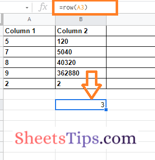
- 3rd Step: Enter the formula “Row(cell_Reference)“. In this example, I am using the formula row(a3).
- 4th Step: Press the “Return” key and you will see the results as shown in the image below.

Row Function for Range of Cells
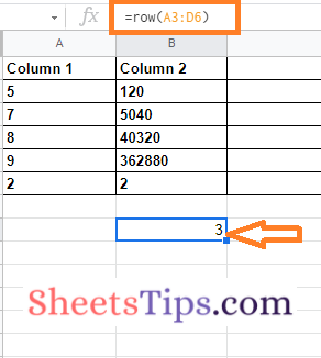
If we want to know the row number for the range of cells in Google Sheets, we can simply use the ROW function. All you have to do this to attach the cell range for which you want to know the row numbers. For example, If I want to know the row number from Range A3 to D6, then our formula will be row(A3:D6). When we use the above formula, our results will be as follows.

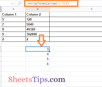
To overcome this issue, we can simply use the Array Formula. Using the Array Formula, we can simply get the results. The array formula to find the row numbers for the range of cells is “=ArrayFormula(A3:D6)”. When we use this formula, you will get the results as shown below.

ROWS Function in Google Sheets
Now that we understood everything about the ROW function in Google Sheets. Now let us understand how to use the ROWS function in the Google Spreadsheet by following the steps outlined below.
- 1st Step: Open the Google Spreadsheet on your device.
- 2nd Step: Now on the homepage, move to the desired cell where you want to get the results of the ROWS function.
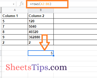
- 3rd Step: Enter the formula “ROWS(cell_range)“. Here in this post, am using an example where I want to know the number of rows between A2 to B6. So my formula here is ROWS(A2:B6).
- 4th Step: After entering the formula, press the “Return” key and you will see the results as shown in the image below.

